
R: XGBoost Solubility Regression
I predicted the aqueous solubility of chemical compounds listed in a public dataset using a basic linear model and an untuned random forest in my previous post. The random forest showed the two models’ best performance, achieving an RMSE of 0.866 and an R^2 of 0.828. In this post, I train an XGBoost model on the same data.
Load the libraries
library(tidyverse)
library(tidymodels)
library(ranger)
library(usemodels)
library(gridExtra)
library(vip)
theme_set(theme_classic())
Load, split, and bootstrap sample the data.
I select the columns I will use as predictors here. I also make the train test split here and initialize the bootstrap sampling.
df <- as_tibble(read.csv("data/delaney-processed.csv")) %>%
  select(
    compound = Compound.ID,
    mw = Molecular.Weight,
    h_bond_donors = Number.of.H.Bond.Donors,
    rings = Number.of.Rings,
    rotatable_bonds = Number.of.Rotatable.Bonds,
    psa = Polar.Surface.Area,
    solubility = measured.log.solubility.in.mols.per.litre
)

set.seed(123)

split <- initial_split(df)
train_data <- training(split)
test_data <- testing(split)
train_boot <- bootstraps(train_data, times = 5)
Get boilerplate for an XGBoost regression.
I leverage usemodels to get the boilerplate code for an XGBoost model.
usemodels::use_xgboost(solubility ~ mw + h_bond_donors + rings + rotatable_bonds + psa, data = train_data)## xgboost_recipe <-
## recipe(formula = solubility ~ mw + h_bond_donors + rings + rotatable_bonds +
## psa, data = train_data) %>%
## step_zv(all_predictors())
##
## xgboost_spec <-
## boost_tree(trees = tune(), min_n = tune(), tree_depth = tune(), learn_rate = tune(),
## loss_reduction = tune(), sample_size = tune()) %>%
## set_mode("regression") %>%
## set_engine("xgboost")
##
## xgboost_workflow <-
## workflow() %>%
## add_recipe(xgboost_recipe) %>%
## add_model(xgboost_spec)
##
## set.seed(72581)
## xgboost_tune <-
## tune_grid(xgboost_workflow, resamples = stop("add your rsample object"), grid = stop("add number of candidate points"))Assemble the model
Using the boilerplate suggestion above as a guide, I follow the steps below to prepare the XGBoost model for training.
First, I make the recipe.
The recipe unites the data, formula, and preprocessing steps. Here, I use all the predictors. While all the predictors have non-zero variance, I still place the step_zv preprocessing step to remove zero-variance predictors as a best practice suggested by the boilerplate.
xgboost_recipe <-
  recipe(formula = solubility ~ mw + h_bond_donors + rings + rotatable_bonds +
    psa, data = train_data) %>%
  step_zv(all_predictors())
Second, I make the spec.
The specification sets the engine as XGBoost, the mode as regression, and specifies the hyperparameters needing tuning.
xgboost_spec <-
  boost_tree(trees = tune(), min_n = tune(), tree_depth = tune(), learn_rate = tune(),
    loss_reduction = tune(), sample_size = tune()) %>%
  set_mode("regression") %>%
  set_engine("xgboost")
Third, I make the workflow.
The workflow ties the spec and recipe together.
xgboost_workflow <-
  workflow() %>%
  add_recipe(xgboost_recipe) %>%
  add_model(xgboost_spec)
Fourth, I tune XGBoost
I set a random seed for reproducibility and enable parallel processing, keeping the default of using half the available cores. Then, I tune based on a grid search of 200 points.
set.seed(123)
doParallel::registerDoParallel()

xgboost_tune <-
  tune_grid(xgboost_workflow, resamples = train_boot, grid = 20)
Evaluate the model
First, I plot performance metrics during the model tuning.
Figure 1 reflects the RMSE and R^2 performance metrics during the tuning process.
autoplot(xgboost_tune) +
  theme_gray()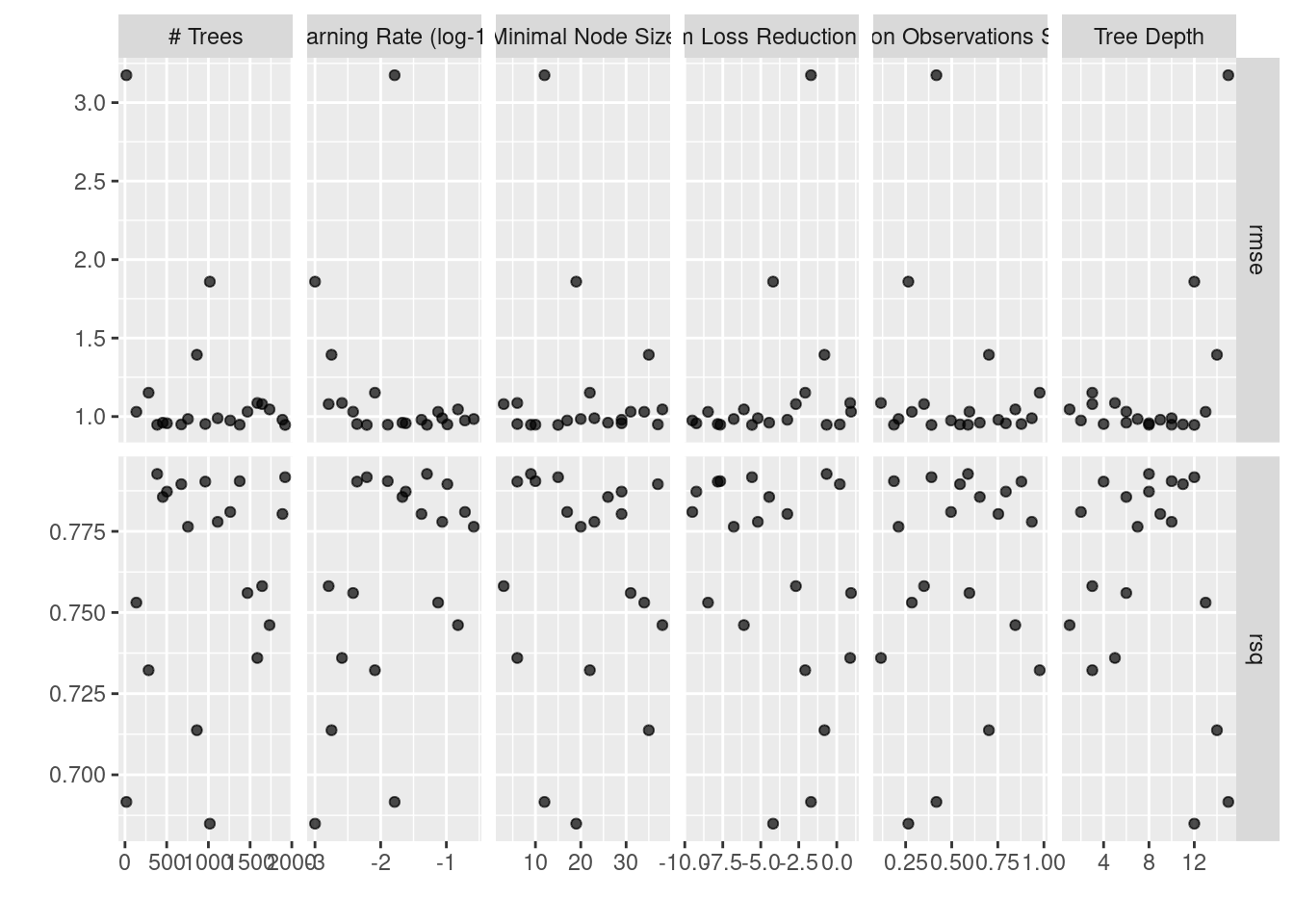
Figure 1: XGBoost Tuning Session
Second, I finalize the workflow.
Workflow finalization selects the best performing hyperparameters based on the RMSE metric.
final_xgb <- xgboost_workflow %>%
  finalize_workflow(select_best(xgboost_tune, metric = "rmse"))
Third, I fit and collect predictions from the best-performing model.
In Figure 2, I plot the predictions with a trend line in the plot to see how well the model behaves on the test data.
solubilty_fit <- last_fit(final_xgb, split)
metrics <- collect_metrics(solubilty_fit)
knitr::kable(metrics)| .metric | .estimator | .estimate | .config |
|---|---|---|---|
| rmse | standard | 0.9204040 | Preprocessor1_Model1 |
| rsq | standard | 0.8094534 | Preprocessor1_Model1 |
collect_predictions(solubilty_fit) %>%
  ggplot(aes(.pred, solubility)) +
  geom_point(alpha = 0.4) +
  stat_smooth(method = "lm", se = FALSE)
## `geom_smooth()` using formula 'y ~ x'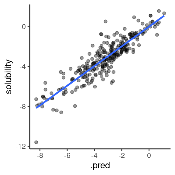
Figure 2: Actual vs predicted solubility
Finally, I check the variable importance.
In Figure 3 of variable importance, molecular weight is the most critical predictor of solubility for the XGBoost model.
final_xgb %>%
  fit(data = train_data) %>%
  pull_workflow_fit() %>%
  vip(geom = "point")
## Warning: `pull_workflow_fit()` was deprecated in workflows 0.2.3.
## Please use `extract_fit_parsnip()` instead.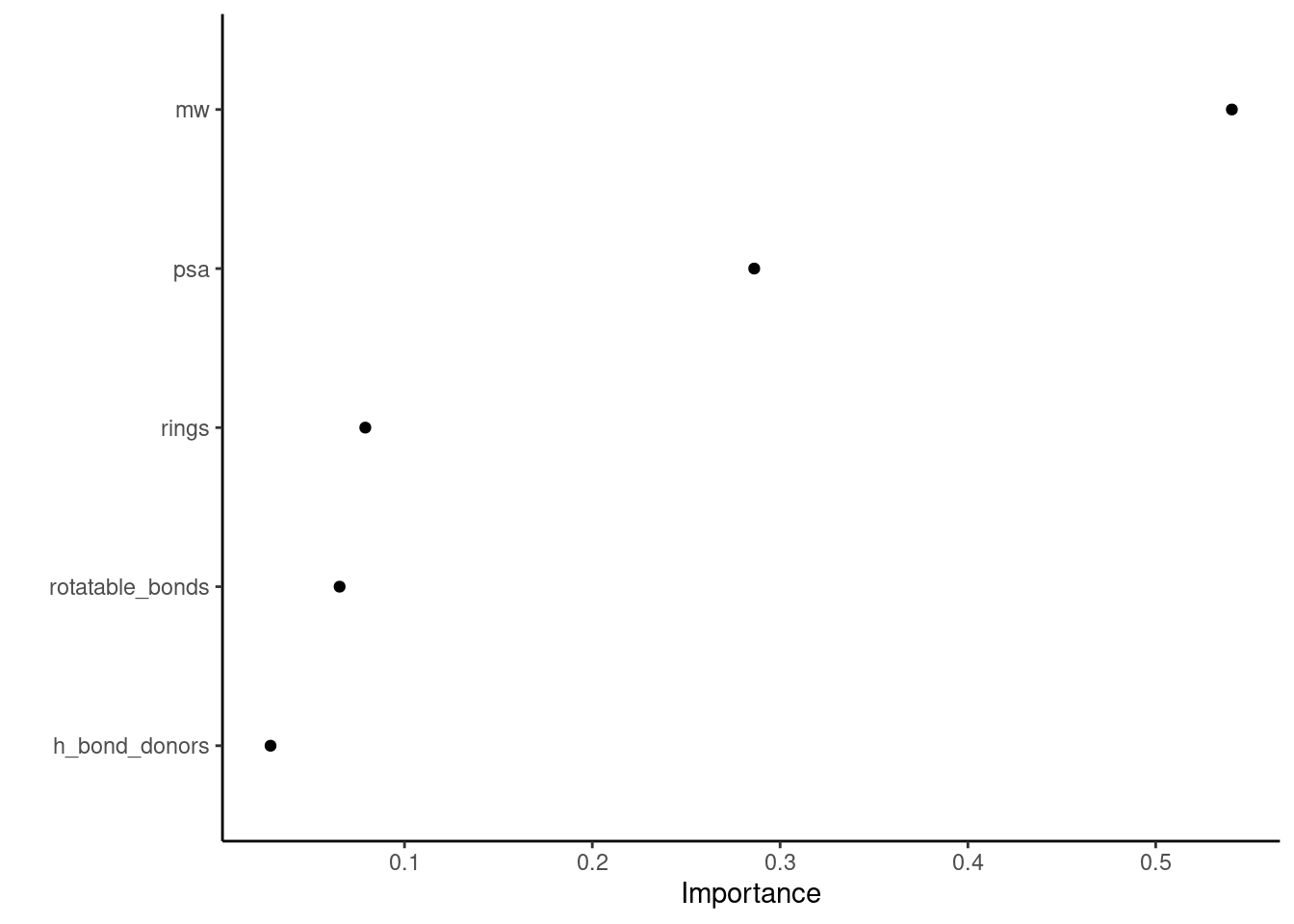
Figure 3: Variable importance
Figure 4 shows how molecular weight tends to increase as the number of features on a molecule increase.
alpha = 0.1
p1 <- ggplot(df, aes(x = psa, y = mw)) +
  geom_jitter(alpha = alpha) +
  geom_smooth(method = "lm", se = FALSE) +
  labs(title = "(a)") +
  theme_minimal()

p2 <- ggplot(df, aes(x = solubility, y = mw)) +
  geom_jitter(alpha = alpha) +
  geom_smooth(method = "lm", se = FALSE) +
  labs(title = "(b)") +
  theme_minimal()

p3 <- ggplot(df, aes(x = h_bond_donors, y = mw)) +
  geom_jitter(alpha = alpha, width = 0.1) +
  geom_smooth(method = "lm", se = FALSE) +
  labs(title = "(c)") +
  theme_minimal()

p4 <- ggplot(df, aes(x = rings, y = mw)) +
  geom_jitter(alpha = alpha, width = 0.1) +
  geom_smooth(method = "lm", se = FALSE) +
  labs(title = "(d)") +
  theme_minimal()

p5 <- ggplot(df, aes(x = rotatable_bonds, y = mw)) +
  geom_jitter(alpha = alpha, width = 0.1) +
  geom_smooth(method = "lm", se = FALSE) +
  labs(title = "(e)") +
  theme_minimal()

grid.arrange(p1, p2, p3, p4, p5, nrow = 3)
## `geom_smooth()` using formula 'y ~ x'
## `geom_smooth()` using formula 'y ~ x'
## `geom_smooth()` using formula 'y ~ x'
## `geom_smooth()` using formula 'y ~ x'
## `geom_smooth()` using formula 'y ~ x'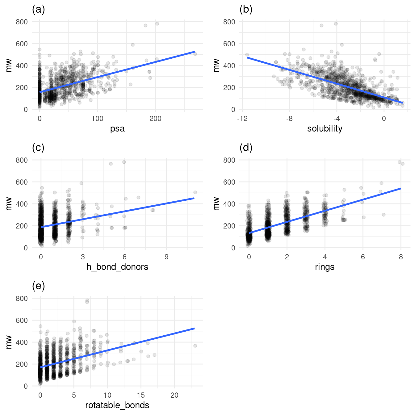
Figure 4: Relationship of molecular weight to other variables
Conclusion
Perhaps the XGBoost model’s perfomance could be improved even further by either increasing the number of sample points on the hyperparameter grid or by using a more intelligent sampling method, such as latin hypercube.
