R: Predicting chemical compound solubility with R, tidyverse, and mlr
Aqueous solubility (ability to dissolve in water) is an important property of a chemical compound that is important in the laboratory. While it is possible to determine these solubilities through physical experiments, let’s assume for this tiny project that such experiments are prohibitively expensive. This presents an interesting predictive modeling problem: given a known chemical structure, can the aqueous solubility of a compound be predicted without physical experiments? This was the question proposed by Delaney in 2004 (Delaney, 2004) in a study that created a simple regression model that took SMILES strings (a data format to store the structure of chemical compounds), extracted features from these data and created a regression model to predict solubility. This paper has been cited over 140 times in the chemistry literature.
The data forthis study come from the deepchem.io project. Here are some compounds in the dataset that may be recognizable with links to Wikipedia:
| Compound name | Description |
|---|---|
| Sucrose | Sugar |
| Erythritol | Sugar substitute |
| Caffiene | I drank too much of it right now… |
| Octane | Component of gasoline |
| Fructose | Component of high fructose corn syrup |
My study here does not seek to replicate the original model from 2004; rather, it is focused on finding if a simple feature selection process (from domain knowledge of chemistry) and a simple predictive model (logistic regression) can do a simple classification of solubilities of compounds: Is the solubility of a compound above or below a certain threshold?
The model in this tiny study has an accuracy of 84% with an AUROC of 88%.
Methods
The original study from 2004 found that the molecular weight and number of rotatable bonds were key predictors of solubility. Solubility was measured in log(g/mol). I used these two variables and a third, polar surface area, as predictor variables, as shown in the table below:
| Variable name | Units | Description |
|---|---|---|
| Molecular Weight | g / mol | the molecular weight of the compound |
| Number of Rotatable Bonds | unitless | The number of rotatable bonds in the compund, as calculated by the patterns in the SMILES string [!X1]-,)- [$([C.;X4])]-&!@[$([C.;X4])]-[!X1], [!X1]:c-&!@[$([C.;X4])]-[!X1], [!X1]-,)C-&!@[$([N.;X4])]-[!X1], [!X1]-[$([C.;X4])]-&!@[$([N.;X3])]- [!X1], [!X1]-[$([C.;X4])]-&!@[$([O.;X2])]-[!X1] |
| Polar Surface Area | Å2 | The surface area of the polar atoms of the compound. See Wikipedia for details |
Each observation in the dataset represents one compound. To each observation, I added a variable called solubility.above.or.below.median. The class labels have the following meaning.
| Class | Relation to median solubility | Test outcome | Description |
|---|---|---|---|
| 1 | > | positive | Solubility greater than the median |
| 0 | <= | negative | Soubility equal to or less than the median |
For the model, I used R, the mlr machine learning package, and tidyverse packages for data manipulation.
Exploratory analysis of the data
I used a train test split with 75% of the observations going to the training data with 25% held out for the test data. The counts of the classes in the training data are:
| solubility.above.or.below.median | n |
|---|---|
| 0 | 419 |
| 1 | 427 |
The counts of the classes in the test data are:
| solubility.above.or.below.median | n |
|---|---|
| 0 | 146 |
| 1 | 136 |
Distributions of predictor variables

Figure 1: Histograms of predictor variables
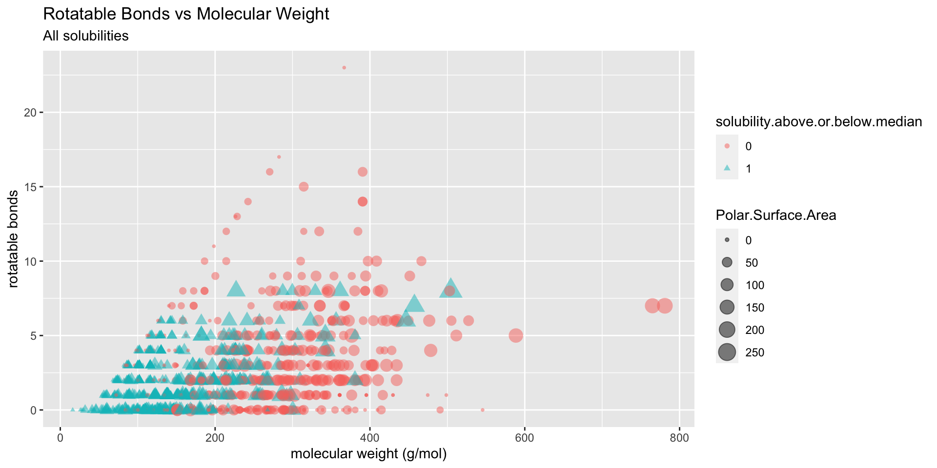
To get a sense for where various levels of solubility fall in relation to one another, I plotted solubility class by rotatable bonds, molecular weight, and polar surface area:

Figure 2: Distribution of solubilitiy classes
Results
I trained and tested the logistic regression model with repeated k-fold cross validation, using 20 shuffles of the training data, with each shuffle in 10 folds. This created 200 logistic regression models from the original training data. This led to the accuracy, false positive rate, and false negative rate in the table below:
| FALSE | |
|---|---|
| acc.test.mean | 0.8378149 |
| fpr.test.mean | 0.1283389 |
| fnr.test.mean | 0.1966551 |
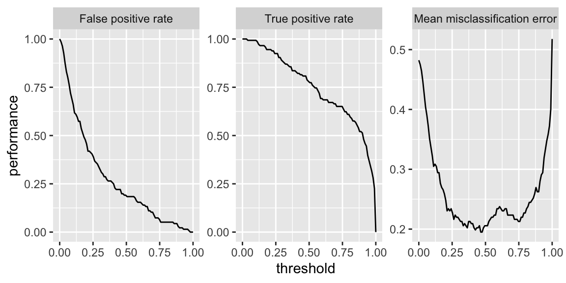
Finally, I pulled out the first model of the 200 created and plotted performance metrics as a function of logistic regression threshold:
## Warning in makeTask(type = type, data = data, weights = weights, blocking =
## blocking, : Provided data is not a pure data.frame but from class tbl_df, hence
## it will be converted.
Figure 3: Performance curves for first logistic regression model
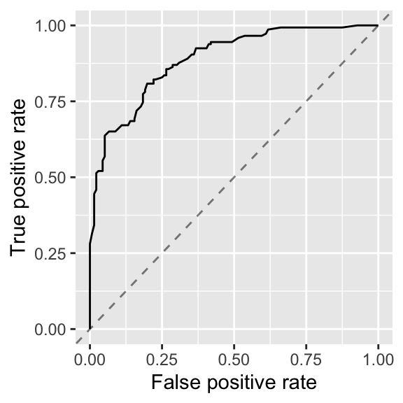
Finally, I made the ROC curve plot:

Figure 4: ROC for first logistic regression model
The AUROC of this model is 89% when the ROC curve is calculated on test data.
Discussion and Conclusion
I’m going to tip the conclusion in this toy model’s favor by assuming that solubility experiments are costly, but not impossible. If the goal of our imaginary experiment is to find and confirm compounds that have solubilities greater than the median, and are willing to experimentally test and eliminate compounds that are below the median, the false positive rate of 13% might be good enough. However, if the goal was to find compounds less than or equal to the median, then with a false negative rate of 20% would result in a lot of unneeded tests.
An AUROC of 89% for a logistic regression is OK. But the false positive rate and false negative rate would make me think twice about using this model to help guide experiments.