
Python: StretchDyn: Molecular dynamics with stretch energy
Molecular dynamics models the motion of atoms within molecules using classical mechanics. Many resources exist online and in print on molecular mechanics. I wanted to learn more about molecular mechanics by implementing it in Python code. Yet, when I searched for resources to lead me in writing my code, I found them scattered online. Pulling them together into a cohesive whole was difficult. In this post, I make a simple molecular dynamics simulation using velocity Verlet integration in Python and compare its results to empirical and analytical values.
I use the diatomic 1H35Cl for the study because its force field consists of only stretch energy. Also, I modeled it using numeric integration, not an analytical solution. I used numeric integration because such an approach could scale to a more complex firce field in the future.
The accompanying source code is at https://github.com/akey7/StretchDyn
Methods
The world of molecules is small with short time periods. To keep the orders of magnitude usable in the code, I use the following units:
Units
| Measure | Unit | mks |
|---|---|---|
| Distance | Angstroms (Å) | \[ 1 \times 10^{-10} m \] |
| Time | femtoseconds (fs) | \[ 1 \times 10^{-15} s \] |
| Mass | atomic mass unit (amu) | \[ 1.66 \times 10^{-27} kg \] |
| Spring constant | \[ \frac{1 \times 10^{-10} N}{Å} \] | N / m |
Variables
For each atom or pairs of atoms, these variables give their positions and velocities:
| Variable | Description | Unit |
|---|---|---|
| \[ \mathbf r_1, \mathbf r_2, ..., \mathbf r_n \] | Positions of the atoms as 3-dimensional vectors | Å |
| \[ \mathbf v_1, \mathbf v_2, ..., \mathbf v_n \] | Velocities of the atoms as 3-dimensional vectors | Å / fs |
| \[ R_{AB} \] | Radius between atoms 1 and 2 | Å |
| \[ \mathbf{F} \] | Force |
Following the notation of Hinchliffe (pp. 53-54), the parameters for the stretch energy of the force field are:
| Force field parameter | Description | Unit |
|---|---|---|
| \[ R_{e,AB} \] | Equilibrium radius between atoms A and B. | Å |
| \[ k_{AB} \] | Force constant for stretch energy between atms A and B | N / m |
Velocity Verlet
I use velocity Verlet algorithm Velocity Verlet as described in Wikipedia useful for doing the numeric integration steps. For each atom, the code performs the following sequence of calculations in the algorithm.
| Step | Formula |
|---|---|
| Calculate next position | \[ \mathbf{r}(t + \Delta t) = \mathbf{r}(t) + \mathbf{r}(t) \Delta t + \mathbf{a}(t) \Delta t^2 \] |
| Calculate acceleration from net force | \[ \mathbf{a}(t + \Delta t) = \frac{\mathbf{F}(t)}{m}\] |
| Calculate next velocity | \[ \mathbf{v}(t + \Delta t) = \mathbf{v}(t) + \frac{1}{2} (\mathbf{a}(t) + \mathbf{a}(t + \Delta t)) \Delta t\] |
Stretch potential
The stretch potential I use follows Hooke’s law as found in Hinchliffe (p. 54):
\[ U_{AB} = \frac{1}{2} k_{AB} (R_{AB} - R_{e,AB})^2 \]
There are other stretch potentitals available to use (Hinchliffe p. 54). One option is to use anharmonic terms. Another option is to use a Morse potential. I chose the wimple harmonic potential because of its simplicity for the model.
The derivative to compute its gradient is:
\[ \frac{dU}{dR} = \frac{1}{2} k_{AB} (2R_{AB} - 2R_{e,AB}) \]
HCl Properties
I used following values for the variables in the simulation:
| Variable | Quantity | Units | Notes |
|---|---|---|---|
| \[ R_{AB} \] | \[ 1.27 \] | \[ Å \] | |
| \[ k_{AB} \] | \[ 8.15 \times 10^{-4} \] | \[ \frac{amu \times Å}{fs^{2}} \] | Converted from 481 N/m |
| \[ \Delta t \] | \[ 1 \] | \[ fs \] |
I experimented with different orders of magnitude for the force constant until I arrived as close as I could to the vibrational frequency of analytially calcuated 1H35Cl. My (admittedly weak) justification for this is that force field parameters are often not exactly the same as the actual parameters (Jensen pp 24-27, p 57).
Results
For the results, I’ll first look at the qualititaive aspect of the calculations: Is the motion what I would expect from a harmonic oscillator? Then I will look at the quantitative aspect: Is the vibrational frequency what I would expect from calculations based on the quantum harmonic oscillator?
Qualitative checks: Is the motion what we would expect?
Because I placed both the H and Cl atoms along the x axis, I simply plotted their displacement along the x axis. As I would expect there are sinusodial motions for both H and Cl. The amplitude of the motion of H is greater because H is a much lighter atom than Cl.
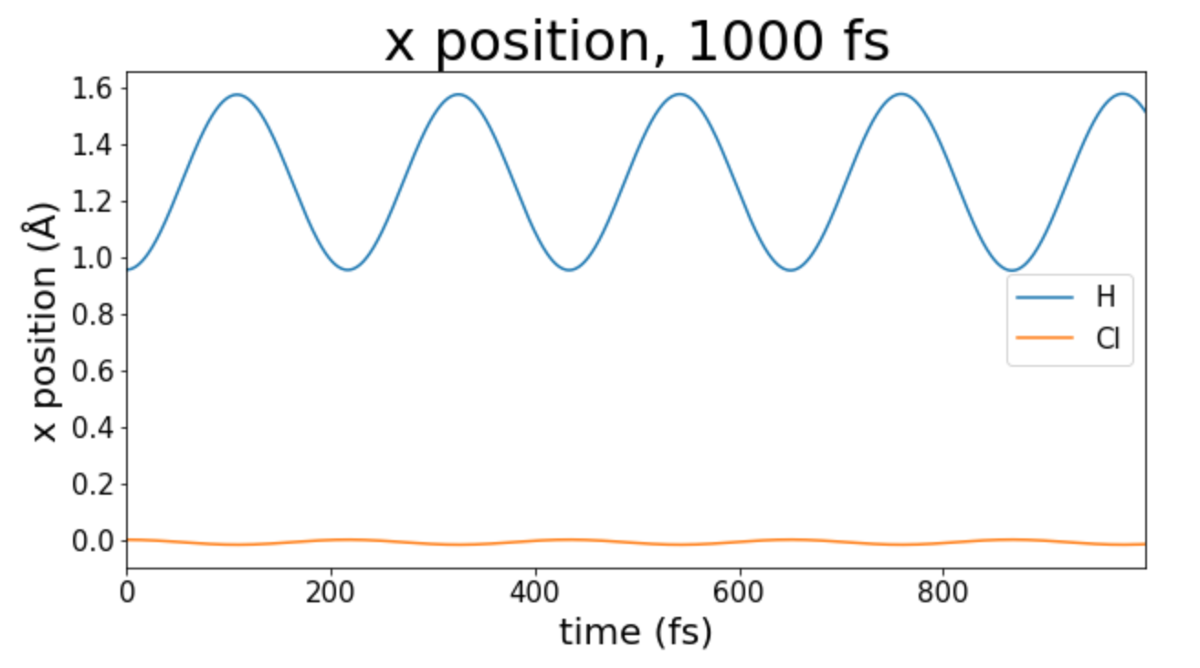
Figure 1: Displacement over many periods of oscillation
Quantitative checks: Are our numbers like what we would calculate from a quantum harmonic oscillator?
The analytically calculated vibrational frequency of 1H35Cl from Atkins and de Paula (p. 453) follows this calculation:
| Step | Calculation |
|---|---|
| Effective mass | \[ m_{eff} = \frac{m_1 m_2}{m_1 + m_2} = \frac{35 \times 1}{35 + 1} = 0.972 amu = 1.63 \times 10^{-27} kg \] |
| Angular frequency | \[ \omega = \sqrt{\frac{k_{AB}}{m_{eff}}} = \sqrt{\frac{480 N/m}{1.63 \times 10^{-27} kg}} = 5.63 \times 10^{14} s^{-1}\] |
| Frequency | \[ \nu = \frac{\omega}{2 \pi} = \frac{5.63 \times 10^{14} s^{-1}}{2 \pi} = 896 THz \] |
What is the vibrational frequency of my simulation?
To start, I find the length of one period of oscillation of H.
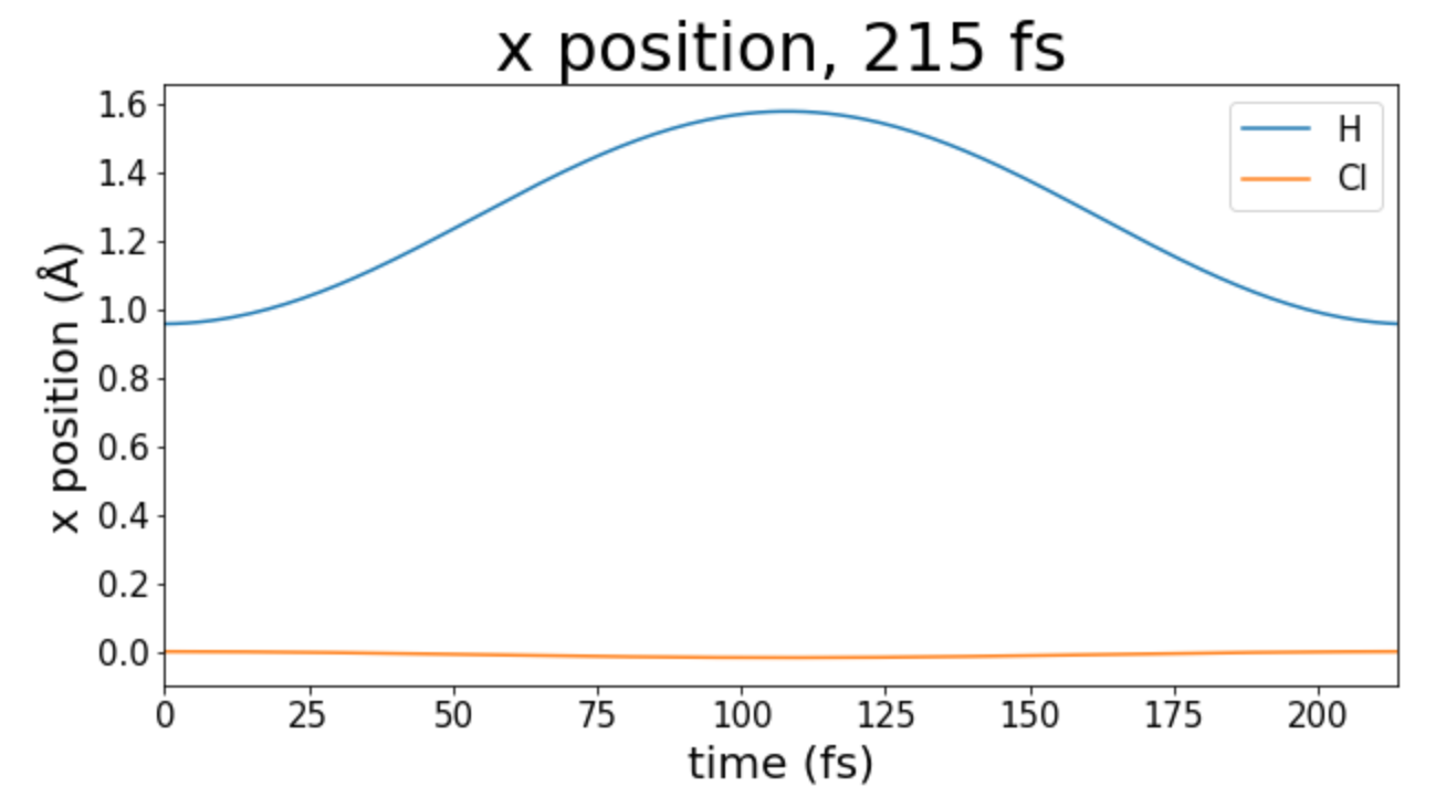
Figure 2: One period of oscillation
That means the period is 215 fs. That makes the frequency
\[ \nu = \frac{1}{T} = \frac{1}{215 \times 10^{-15} s} = 4.65 \times 10^{12} s^{-1} \]
Which is off by two order of magnitude. Disappointing!
Discussion and future work
The good result is the motion of the molecule is what it should be. The problem, however, is that the vibrational frequency is off.
If I were to work on correcting this, I might try the following changes to see if I obtained different results:
- Another numeric integration algorithm, such as leapfrog
- Another stretch potential, such as a Morse potential or a potential that incorporated anharmonic terms.
- A shorter delta t in the numeric integration so I could push push the period to be even shorter with higher stretch potentials.
- Do everything in meters, kilograms, seconds units so I wouldn’t have strange unit conversions.
Overall, I wouldn’t use this for any research purposes (obviosuly!) It has been an educational project to write, but I will stick with established molecular dynamics codes for any serious computational work.
Works Cited
- Atikins, Peter and Julio de Paula. Physical Chemistry, 8th Ed. W.H. Freeman and Company, 2006
- Jensen, Frank. Introduction to Computational Chemistry, 3rd Ed.. Wiley, 2017
- Hinchliffe, Alan. Molecular Modeling for Beginners, 2nd Ed.. Wiley, 2008
