
R: Deep Learning Organic Chemistry Again
Introduction
In my post “Python: Deep Learning Organic Chemistry," I trained a convolutional neural network to recognize a diagram of a benzene ring, which is a crucial structure in many organic chemistry molecules. The classification problem I posed to the convnet was a binary classification to separate diagrams of molecules that contain a benzene ring from those that do not. Using Python, TensorFlow, and Keras, my experiment proceeded in three steps:
- I split 410 grayscale images into testing, training, and validation datasets.
- I trained a convnet base and the dense classifier layers on top of that base from scratch.
- I reached a classification accuracy of 73%.
Attempting to train an entire convnet from just 410 images proved problematic, and a small dataset was the primary problem with my first experiment.
In this post (using R, TensorFlow, and Keras), I created a similar classifier trained on the 410 images. However, since I had limited training data, I changed my goal. First, I would split the images into 300 training and 110 validation images. Then, rather than test on a separate testing set, I would look at the misclassifications in the validation set to learn about my model’s weaknesses. Overall, my model achieves 86% validation accuracy. While I am suspicious of this score because the validation accuracy does not converge over successive epochs, I still found the analysis of the misclassifications to be an insightful activity that points to future directions for this study. I include the R code that I used for experiment to reference for future experiments.
Review of the classification problem
Here is a brief overview of the classification problem that I originally wrote in the first post I mentioned above.
A detailed description of the organic chemistry involved in the training, test and validation datasets is beyond the scope of this article; however, a quick explanation about the data, as well as why the data have meaning in chemistry applications, should prove useful in understanding the convnet setup described here. An important part of studying chemical molecules involves breaking them into smaller substructures and analyzing each substructure individually. By understanding how each part works in the entire chemical structure, one can understand the properties of the compound as a whole. One important strucuture in organic chemistry is called a “benzene ring”. When the ring is found in a standalone configuration, with no other atoms surrounding it, it forms the compound benzene.
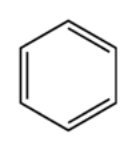 Figure 1: Benzene
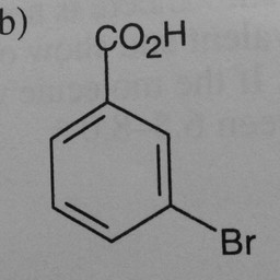
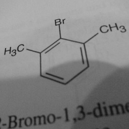
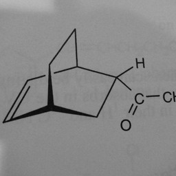
Other parts of a molecule can be attached to these benzene rings, as shown in Figure 2:
 |
 |
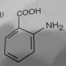 |
Figure 2: Compounds with benzene rings.
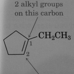
Other compounds do not contain these rings, as seen in the following molecules:
 |
 |
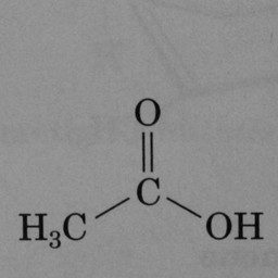 |
Figure 3: Compounds without benzene rings.
The task for the convnet is binary classification to distinguish images of molecules with benzene rings from those without benzene rings.
Training of model
library(keras)
library(tensorflow)
Define where the image datasets are
There is a small dataset of 410 images. Because there are so few images, I will just work with a training and validation set, and I will not use a separate test dataset.
| dataset | benzene ring images | non benzene ring images |
|---|---|---|
| train | 150 | 150 |
| validation | 55 | 55 |
train_dir <- "data/train"
validation_dir <- "data/validation"
Create the image generators
create_generators <- function(test_validation_batch_size) {
  validation_datagen <- image_data_generator(rescale = 1/255)
  train_datagen <- image_data_generator(rescale = 1/255)

  train_generator <- flow_images_from_directory(
    train_dir,
    train_datagen,
    target_size = c(256, 256),
    batch_size = test_validation_batch_size,
    shuffle = FALSE,
    class_mode = "binary"
  )

  validation_generator <- flow_images_from_directory(
    validation_dir,
    validation_datagen,
    target_size = c(256, 256),
    batch_size = test_validation_batch_size,
    shuffle = FALSE,
    class_mode = "binary"
  )

  list(train_generator = train_generator, validation_generator = validation_generator)
}
Define the network
Use VGG16 trained on imagenet for the convolutional layers. Freeze the convolutional layers so that their weights are not adjusted during training. The final layers will be a simple binary classifier made with dense layers.
create_network <- function() {
  conv_base <- application_vgg16(
    weights = "imagenet",
    include_top = FALSE,
    input_shape = c(256, 256, 3)
  )

  conv_base %>% freeze_weights()

  network <- keras_model_sequential() %>%
    conv_base %>%
    layer_flatten() %>%
    layer_dense(units = 256, activation = "relu") %>%
    layer_dense(units = 128, activation = "relu") %>%
    layer_dense(units = 64, activation = "relu") %>%
    layer_dense(units = 1, activation = "sigmoid")

  network %>% compile(
    loss = "binary_crossentropy",
    optimizer = optimizer_rmsprop(learning_rate = 0.5e-5),
    metrics = c("accuracy")
  )

  network
}

convnet_1 <- create_network()
summary(convnet_1)
## Model: "sequential"
## ________________________________________________________________________________
##  Layer (type)                       Output Shape                    Param #
## ================================================================================
##  vgg16 (Functional)                 (None, 8, 8, 512)               14714688
##
##  flatten (Flatten)                  (None, 32768)                   0
##
##  dense_3 (Dense)                    (None, 256)                     8388864
##
##  dense_2 (Dense)                    (None, 128)                     32896
##
##  dense_1 (Dense)                    (None, 64)                      8256
##
##  dense (Dense)                      (None, 1)                       65
##
## ================================================================================
## Total params: 23,144,769
## Trainable params: 8,430,081
## Non-trainable params: 14,714,688
## ________________________________________________________________________________
Fit the network using the training and validation data
Checkpoint every epoch that shows a better val_accuracy than the previously saved checkpoint.
tensorflow::set_random_seed(0)

callbacks_list <- list(
  callback_model_checkpoint(
    filepath = "organicml_checkpoint.h5",
    monitor = "val_accuracy",
    mode = "max",
    save_best_only = TRUE
  )
)

test_validation_batch_size <- 25
generators_1 <- create_generators(test_validation_batch_size = test_validation_batch_size)

fit_history_1 <- convnet_1 %>%
  fit(
    generators_1$train_generator,
    steps_per_epoch = 300/test_validation_batch_size,
    epochs = 50,
    validation_data = generators_1$validation_generator,
    validation_steps = 110/test_validation_batch_size,
    callbacks = callbacks_list
  )
Analyze training history
Analyzing the training history of the model reveals its most significant flaw: the validation accuracy does not converge during training.
plot(fit_history_1)
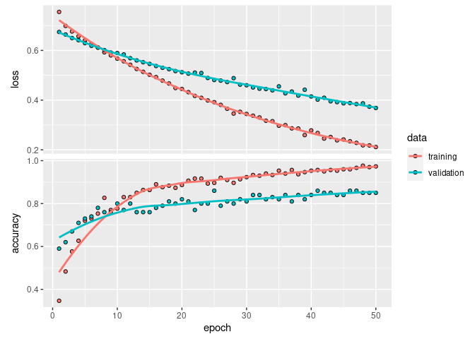
During training, epoch 25 had the maximum validation accuracy of 86%.
Evaluation of model
I evaluated the model from another R markdown notebook that loaded the trained model and performed analytics on it.
library(keras)
library(tibble)
library(dplyr)
library(readr)
Recreate generator for validation images
batch_size <- 10
validation_dir <- "data/validation"

validation_datagen <- image_data_generator(rescale = 1/255)

validation_generator <- flow_images_from_directory(
    validation_dir,
    validation_datagen,
    target_size = c(256, 256),
    batch_size = batch_size,
    shuffle = FALSE,
    class_mode = "binary"
  )
Reload and Evaluate
Reload and evaluate the best model that was saved.
network <- load_model_hdf5("organicml_checkpoint.h5")
network %>% evaluate(validation_generator)
##      loss  accuracy
## 0.5034932 0.8181818
Make a vector of all output from the model
Present each batch of validation images to the network and store the predicted labels. This code is derved from Deep Learning with R Listing 5.17.
predicted <- c()
actual <- c()
i <- 0
while(TRUE) {
  batch <- generator_next(validation_generator)
  inputs_batch <- batch[[1]]
  labels_batch <- batch[[2]]
  predicted <- c(predicted, round(network %>% predict(inputs_batch)))
  actual <- c(actual, labels_batch)
  i <- i + 1
  if (i * batch_size >= validation_generator$samples)
    break
}
Evaluate the errors
Assemble a dataframe that lines up predictions alongside the actual labels and the input image filename.
evaluation_df <- tibble(
    image_filename = validation_generator$filepaths,
    actual = actual,
    predicted = predicted
  )
Compute accuracy, true positive rate (tpr), true negative rate (tnr), false negative rate (fnr), and false positive rate (fpr). Using formulas from https://en.wikipedia.org/wiki/Sensitivity_and_specificity.
network_performance <- evaluation_df %>%
  summarize(
    accuracy = sum(actual == predicted) / n(),
    tpr = sum(actual == 1 & predicted == 1) / sum(actual == 1),
    tnr = sum(actual == 0 & predicted == 0) / sum(actual == 0),
    fpr = sum(actual == 0 & predicted == 1) / sum(actual == 0),
    fnr = sum(actual == 1 & predicted == 0) / sum(actual == 1)
  )
knitr::kable(network_performance)
| accuracy | tpr | tnr | fpr | fnr |
|---|---|---|---|---|
| 0.8181818 | 0.7636364 | 0.8727273 | 0.1272727 | 0.2363636 |
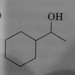
Observe the misclassifications
A class of 1 means that the compound diagram contains a benzene ring and 0 means no benzene ring.
| Diagram | Actual class | Predicted class | What failed |
|---|---|---|---|
 |
0 | 1 | A hexagon without double bonds is not a benzene ring. |
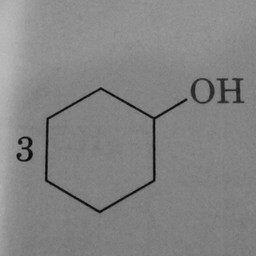 |
0 | 1 | A hexagon without double bonds is not a benzene ring. |
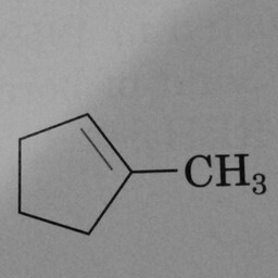 |
0 | 1 | A pentagon with just one double bond is not a benzene ring. |
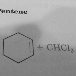 |
0 | 1 | A hexagon with one double bond is not a benzene ring. |
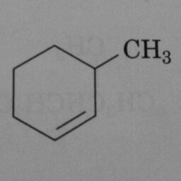 |
0 | 1 | A hexagon with one double bond is not a benzene ring. |
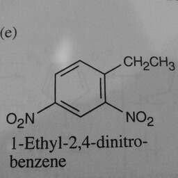 |
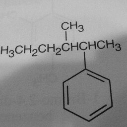
1 | 0 | The network is confused by other groups connected to the benzene ring. |
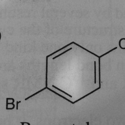 |
1 | 0 | The network is confused by other groups connected to the benzene ring, and there are shadows in this image. |
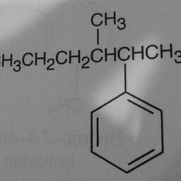 |
1 | 0 | The network is confused by other groups connected to the benzene ring, and there are shadows in this image. |
 |
1 | 0 | The network is confused by other groups connected to the benzene ring, and there are shadows in this image. |
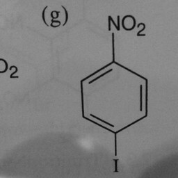 |
1 | 0 | The network is confused by other groups connected to the benzene ring, and there are shadows in this image. |
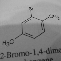 |
1 | 0 | The network is confused by other groups connected to the benzene ring, there are shadows in this image, and the image is slanted. |
 |
1 | 0 | The network is confused by other groups connected to the benzene ring, and there are shadows in this image. |
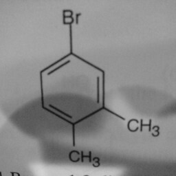
 |
1 | 0 | The network is confused by other groups connected to the benzene ring, there are shadows in this image, and the image is slanted. |
 |
1 | 0 | The network is confused by other groups connected to the benzene ring, there are shadows in this image, and the image is slanted. |
As an interesting note, I found two images that I thought were mislabeled in the input data, so the little network performed better than I thought!
Conclusion
As a follow up to this analysis of the model’s misclassifications, I could take the following steps:
-
Manually recheck the labels on the training images.
-
Preprocess the pictures in a way that minimizes the contrast of the shadows.
-
Augment the training data set with more photos of benzene ring cases that are slanted.
