
R: Deep Learning Organic Chemistry Part 3
Introduction
In my post “R: Deep Learning Organic Chemistry Again,” I trained a convolutional neural network based on VGG16 to recognize a benzene ring diagram, a crucial structure in many organic chemistry molecules. The classification problem I posed to the convnet was a binary classification to separate diagrams of molecules that contain a benzene ring from those that do not. However, near the end of that post, I found images I had mistakenly put in the wrong training and validation folders. My mistake meant I attempted to train and evaluate the convnet on corrupt training data. Oops!
I fixed the training and validation data classifications by moving two images from the non-benzene ring class to the benzene ring class. I then reran the same R as before. With good training and validation data, my model’s performance improved the accuracy, true positive rate (TPR), and false negative rate (FNR) metrics. Interstingly, the true negative rate (TNR) and false positive rate (FPR) became worse.
With corrupt training and validation data:
| accuracy | tpr | tnr | fpr | fnr |
|---|---|---|---|---|
| 0.8181818 | 0.7636364 | 0.8727273 | 0.1272727 | 0.2363636 |
With fixed training and validation data:
| accuracy | tpr | tnr | fpr | fnr |
|---|---|---|---|---|
| 0.8454545 | 0.877193 | 0.8113208 | 0.1886792 | 0.122807 |
While I still had a suboptimal number of images, I am happy that I improved the model’s performance.
Below is the R code that trained and evaluated the model. Following the R code, I manually examine misclassifications in the validation set to see what the model got wrong.
Define where the image datasets are
There is a small dataset of 410 images. Because there are so few images, I will just work with a training and validation set, and I will not use a separate test dataset.
| dataset | benzene ring images | non benzene ring images |
|---|---|---|
| train | 152 | 148 |
| validation | 57 | 53 |
train_dir <- "data/train"
validation_dir <- "data/validation"
Create the image generators
Use data augmentation on the training set, but not the validation set.
Create a function to create the generators. This function will be called twice. The first time will be during training of the first network. The second time will be training the second network.
create_generators <- function(test_validation_batch_size) {
  validation_datagen <- image_data_generator(rescale = 1/255)
  train_datagen <- image_data_generator(rescale = 1/255)

  train_generator <- flow_images_from_directory(
    train_dir,
    train_datagen,
    target_size = c(256, 256),
    batch_size = test_validation_batch_size,
    shuffle = FALSE,
    class_mode = "binary"
  )

  validation_generator <- flow_images_from_directory(
    validation_dir,
    validation_datagen,
    target_size = c(256, 256),
    batch_size = test_validation_batch_size,
    shuffle = FALSE,
    class_mode = "binary"
  )

  list(train_generator = train_generator, validation_generator = validation_generator)
}
Define the network
Use VGG16 trained on imagenet for the convolutional layers. Freeze the convolutional layers so that their weights are not adjusted during training. The final layers will be a simple binary classifier made with dense layers.
First, make a function that can return an initalized network.
create_network <- function() {
  conv_base <- application_vgg16(
    weights = "imagenet",
    include_top = FALSE,
    input_shape = c(256, 256, 3)
  )

  conv_base %>% freeze_weights()

  network <- keras_model_sequential() %>%
    conv_base %>%
    layer_flatten() %>%
    layer_dense(units = 256, activation = "relu") %>%
    layer_dense(units = 128, activation = "relu") %>%
    layer_dense(units = 64, activation = "relu") %>%
    layer_dense(units = 1, activation = "sigmoid")

  network %>% compile(
    loss = "binary_crossentropy",
    optimizer = optimizer_rmsprop(learning_rate = 0.5e-5),
    metrics = c("accuracy")
  )

  network
}
Now use the function to create the network
convnet_1 <- create_network()
## Loaded Tensorflow version 2.7.0
summary(convnet_1)
## Model: "sequential"
## _____________________________________________________________________
##  Layer (type)                  Output Shape               Param #
## =====================================================================
##  vgg16 (Functional)            (None, 8, 8, 512)          14714688
##  flatten (Flatten)             (None, 32768)              0
##  dense_3 (Dense)               (None, 256)                8388864
##  dense_2 (Dense)               (None, 128)                32896
##  dense_1 (Dense)               (None, 64)                 8256
##  dense (Dense)                 (None, 1)                  65
## =====================================================================
## Total params: 23,144,769
## Trainable params: 8,430,081
## Non-trainable params: 14,714,688
## _____________________________________________________________________
Fit the network using the training and validation data
Checkpoint every model that shows a better val_accuracy than the
previous. Stop training when there have been 5 epochs without
improvement to val_accuracy.
tensorflow::set_random_seed(0)

callbacks_list <- list(
  callback_model_checkpoint(
    filepath = "organicml_checkpoint.h5",
    monitor = "val_accuracy",
    mode = "max",
    save_best_only = TRUE
  )
)

test_validation_batch_size <- 25
generators_1 <- create_generators(test_validation_batch_size = test_validation_batch_size)

fit_history_1 <- convnet_1 %>%
  fit(
    generators_1$train_generator,
    steps_per_epoch = 300/test_validation_batch_size,
    epochs = 50,
    validation_data = generators_1$validation_generator,
    validation_steps = 110/test_validation_batch_size,
    callbacks = callbacks_list
  )
Analyze training history
plot(fit_history_1)
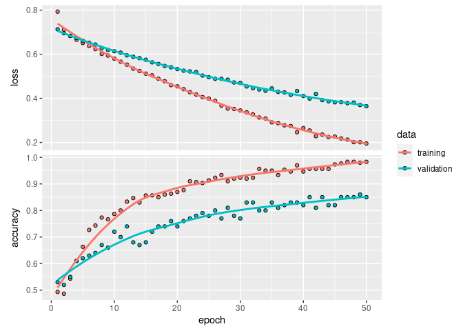
What epoch had the maximum validation accuracy?
max_val_accuracy_1 <- max(fit_history_1$metrics$val_accuracy)
argmax_val_accuracy_1 <- which.max(fit_history_1$metrics$val_accuracy)
cat("Maximum val_accuracy: ", max_val_accuracy_1, "\n")
## Maximum val_accuracy: 0.86
cat("Epoch of maximum validation accuracy: ", argmax_val_accuracy_1, "\n")
## Epoch of maximum validation accuracy: 49
Recreate generator for evaluation images
batch_size <- 10
validation_dir <- "data/validation"

validation_datagen <- image_data_generator(rescale = 1/255)
## Loaded Tensorflow version 2.7.0
validation_generator <- flow_images_from_directory(
    validation_dir,
    validation_datagen,
    target_size = c(256, 256),
    batch_size = batch_size,
    shuffle = FALSE,
    class_mode = "binary"
  )
Reload and Evaluate
Reload and evaluate the best model that was saved.
network <- load_model_hdf5("organicml_checkpoint.h5")
network %>% evaluate(validation_generator)
##      loss  accuracy
## 0.3878245 0.8454546
Make a vector of all output from the model
Present each batch of images from the generator (it has already been iterated over once) and obtain the output of the sigmoid activation function that is the last layer of the network.
predicted <- c()
actual <- c()
network_input <- c()
i <- 0
while(TRUE) {
  batch <- generator_next(validation_generator)
  inputs_batch <- batch[[1]]
  labels_batch <- batch[[2]]
  predicted <- c(predicted, round(network %>% predict(inputs_batch)))
  actual <- c(actual, labels_batch)
  network_input <- c(network_input, inputs_batch)
  i <- i + 1
  if (i * batch_size >= validation_generator$samples)
    break
}
Compute the error rate
Assemble a dataframe that lines up predictions alongside the actual labels and the input image filename.
evaluation_df <- tibble(
    image_filename = validation_generator$filepaths,
    actual = actual,
    predicted = predicted
  )
Compute accuracy, true positive rate (tpr), true negative rate (tnr), false negative rate (fnr), and false positive rate (fpr). Using formulas from https://en.wikipedia.org/wiki/Sensitivity_and_specificity.
network_performance <- evaluation_df %>%
  summarize(
    accuracy = sum(actual == predicted) / n(),
    tpr = sum(actual == 1 & predicted == 1) / sum(actual == 1),
    tnr = sum(actual == 0 & predicted == 0) / sum(actual == 0),
    fpr = sum(actual == 0 & predicted == 1) / sum(actual == 0),
    fnr = sum(actual == 1 & predicted == 0) / sum(actual == 1)
  )
knitr::kable(network_performance)
| accuracy | tpr | tnr | fpr | fnr |
|---|---|---|---|---|
| 0.8454545 | 0.877193 | 0.8113208 | 0.1886792 | 0.122807 |
Create a csv of failed classification attempts
evaluation_df %>%
  filter(actual != predicted) %>%
  write_csv("organicml-evaluation-failures.csv")
Observe the misclassifications
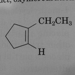
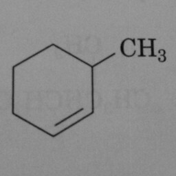
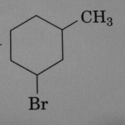
A positive class of 1 means that the compound diagram contains a benzene ring and a negative class of 0 means no benzene ring.
| Diagram | Actual class | Predicted class | What failed |
|---|---|---|---|
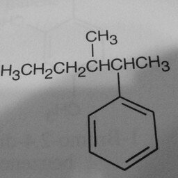 |
1 | 0 | Substituent groups attached confused the convnet. |
 |
1 | 0 | Substituent groups attached confused the convnet. |
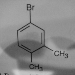 |
1 | 0 | Substituent groups attached confused the convnet. |
 |
1 | 0 | Substituent groups attached confused the convnet. |
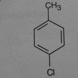 |
1 | 0 | Substituent groups attached confused the convnet. |
 |
1 | 0 | Substituent groups attached confused the convnet. |
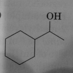 |
0 | 1 | A prominent and well-positioned hexagon without double bonds confused the convnet. |
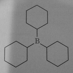 |
0 | 1 | Three prominent and well-positioned hexagons without double bonds confused the convnet. |
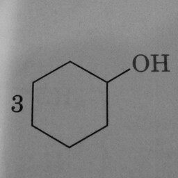 |
0 | 1 | A prominent and well-positioned hexagon without double bonds confused the convnet. Could the “3” have been misinterpreted as a double bond? |
 |
0 | 1 | A prominent and well-positioned hexagon without double bonds confused the convnet. Could the “3” have been misinterpreted as a double bond? |
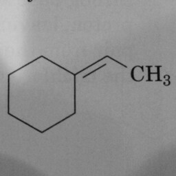 |
0 | 1 | A prominent and well-positioned hexagon without double bonds confused the convnet…but, there is one double bond in this image, just not in the hexagon. |
|
0 | 1 | The hexagon should have had 3 double bonds to be in the positive class. |
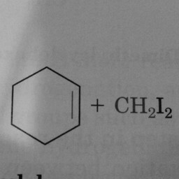 |
0 | 1 | The hexagon should have had 3 double bonds to be in the positive class. |
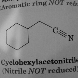 |
0 | 1 | The convnet probably mistook the triple-bonded C N atoms for a double bond. |
 |
0 | 1 | Again, there need to be three double bonds in the hexagon for the postive class. |
 |
0 | 1 | A prominent and well-positioned hexagon without double bonds confused the convnet. |
Conclusion
To improve the network (yet again) I would provide more training images and, in particular, benzene rings with substitutent groups that are labeled in the positive class.
