
R: Milk quality binary classification
Overview
I was looking for a dataset on which to train a binary classifier, and I found data for dairy milk quality prediction on Kaggle. Posted by Shrijayan Rajendran and located at https://www.kaggle.com/datasets/cpluzshrijayan/milkquality, it has a single outcome variable that classifies milk into three qualities: “low,” “medium,” and “high.” Seven predictor variables accompany these quality ratings. Conveniently, there are no missing values in the dataset.
Ultimately, I converted the three qualities into new categories with just two types. I then trained a logistic regression which achieved the following metrics:
| Metric | Value |
|---|---|
| accuracy | 85% |
| sensitivity | 90% |
| specificty | 77% |
| ROC AUC | 0.92 |
The rest of this post describes my methods and next steps that might improve the model.
Methods
R libraries I used
I used R with the tidyverse tools for data import and preprocessing, along with tidymodels for creating a logistic regression model and assessing its performance.
Initial data load
In the dataset, there are 1,059 observations with eight variables each. There is no missing data.
milk_raw <- read_csv("data/milknew.csv")## Rows: 1059 Columns: 8
## ── Column specification ───────────────────────────────────────────────────────────────────────────────────────────────────────────────────────────────────────────────────────────────────
## Delimiter: ","
## chr (1): Grade
## dbl (7): pH, Temprature, Taste, Odor, Fat, Turbidity, Colour
##
## ℹ Use `spec()` to retrieve the full column specification for this data.
## ℹ Specify the column types or set `show_col_types = FALSE` to quiet this message.knitr::kable(head(milk_raw))| pH | Temprature | Taste | Odor | Fat | Turbidity | Colour | Grade |
|---|---|---|---|---|---|---|---|
| 6.6 | 35 | 1 | 0 | 1 | 0 | 254 | high |
| 6.6 | 36 | 0 | 1 | 0 | 1 | 253 | high |
| 8.5 | 70 | 1 | 1 | 1 | 1 | 246 | low |
| 9.5 | 34 | 1 | 1 | 0 | 1 | 255 | low |
| 6.6 | 37 | 0 | 0 | 0 | 0 | 255 | medium |
| 6.6 | 37 | 1 | 1 | 1 | 1 | 255 | high |
Preprocessing
I only performed one preprocessing step to create a binary classification from three original classes. Because there are three classes in the data, and I could only use two for a binary classifier, I combined the initial “high” and “medium” qualities into a new category I called “good” and the original “low” quality into a new category called “bad.” I then used these new categories to train the binary classifier. My positive event is finding milk of “good” quality, so I make “good” the first factor level for the outcome variable.
milk_clean <- milk_raw %>%
  transmute(
    pH,
    Temperature = Temprature,
    Odor,
    Fat,
    Turbidity,
    Taste,
    Color = Colour,
    Quality = factor(
      case_when(
        Grade == "high" ~ "good",
        Grade == "medium" ~ "good",
        Grade == "low" ~ "bad"
      ),
      levels = c("good", "bad")
    )
  )

knitr::kable(head(milk_clean))| pH | Temperature | Odor | Fat | Turbidity | Taste | Color | Quality |
|---|---|---|---|---|---|---|---|
| 6.6 | 35 | 0 | 1 | 0 | 1 | 254 | good |
| 6.6 | 36 | 1 | 0 | 1 | 0 | 253 | good |
| 8.5 | 70 | 1 | 1 | 1 | 1 | 246 | bad |
| 9.5 | 34 | 1 | 0 | 1 | 1 | 255 | bad |
| 6.6 | 37 | 0 | 0 | 0 | 0 | 255 | good |
| 6.6 | 37 | 1 | 1 | 1 | 1 | 255 | good |
Model setup and training
I used 793 rows for training and 266 rows for testing. First, I set up a logistic regression binary classifier using R’s glm function. Then, I predicted the class (stored as the variable Quality) using every other variable.
milk_split <- initial_split(milk_clean, prop = 0.75, strata = Quality)

logistic_model <- logistic_reg() %>%
  set_engine("glm") %>%
  set_mode("classification")

logistic_last_fit <- logistic_model %>%
  last_fit(Quality ~ ., split = milk_split)
Results
ROC AUC and accuracy metrics
logistic_last_fit %>%
  collect_metrics() %>%
knitr::kable()| .metric | .estimator | .estimate | .config |
|---|---|---|---|
| accuracy | binary | 0.8308271 | Preprocessor1_Model1 |
| roc_auc | binary | 0.9195382 | Preprocessor1_Model1 |
ROC curve and mosaic plot
logistic_last_fit_results <- logistic_last_fit %>%
  collect_predictions()

logistic_last_fit_results %>%
  roc_curve(truth = Quality, .pred_good) %>%
  autoplot()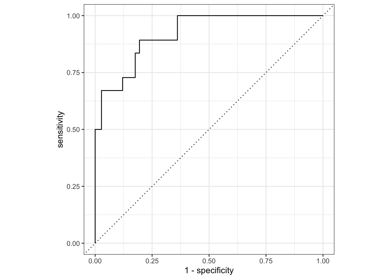
logistic_last_fit_results %>%
  conf_mat(truth = Quality, estimate = .pred_class) %>%
  autoplot(type = "mosaic")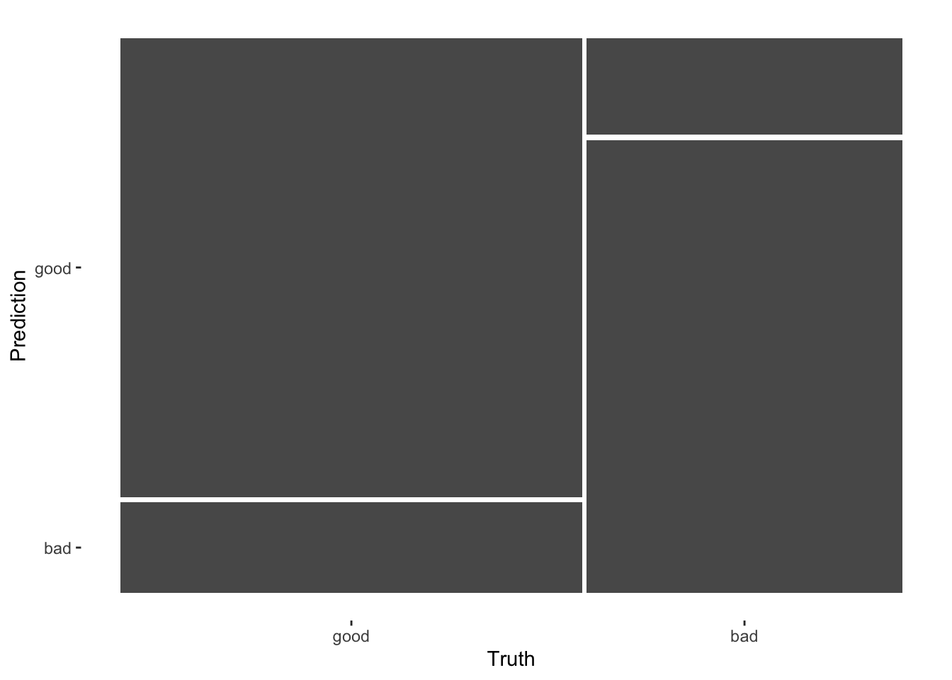
The ROC plot shows the ROC AUC of 0.92 visually. In the mosaic plot, we see the sensitivity of 90% is better than the specificity of 77%.
All metrics
logistic_last_fit_results %>%
  conf_mat(truth = Quality, estimate = .pred_class) %>%
  summary() %>%
knitr::kable()| .metric | .estimator | .estimate |
|---|---|---|
| accuracy | binary | 0.8308271 |
| kap | binary | 0.6528221 |
| sens | binary | 0.8354430 |
| spec | binary | 0.8240741 |
| ppv | binary | 0.8741722 |
| npv | binary | 0.7739130 |
| mcc | binary | 0.6537762 |
| j_index | binary | 0.6595171 |
| bal_accuracy | binary | 0.8297586 |
| detection_prevalence | binary | 0.5676692 |
| precision | binary | 0.8741722 |
| recall | binary | 0.8354430 |
| f_meas | binary | 0.8543689 |
Conclusion and next steps
I was happy with how simple it was to set up the logistic model using tidymodels and achieve decent results with such a basic model. However, there is room for improvement in terms of specificity. The next step would be to try more complex binary classification models to determine if they can achieve better metrics.
