R: PDB Data Exploration
PDB Data Exploration
The Protein DataBank (PDB) stores files that contain the structure of “proteins, nucleic acids, and complex assemblies.” These structures are essential tools for research in structural biology, biochemistry, and related fields. I was recently browsing Kaggle for datasets and found a scrape of PDB data up to the year 2018 by Shahir. The data included sequence information as well as metadata about those sequences. Kaggle suggests these data as a multi-class classification exercise. For this post, I am interested in exploring the metadata to find the data stored in the database and trends in how researchers collected those data.
Include libraries and set plot theme.
Libraries
suppressPackageStartupMessages(library(dplyr))
suppressPackageStartupMessages(library(tidyr))
suppressPackageStartupMessages(library(readr))
suppressPackageStartupMessages(library(ggplot2))
Set theme and dplyr options
theme_set(theme_minimal())
options(dplyr.summarise.inform = FALSE)
Load the dataset
pdb <- read_csv("data/pdb_data_no_dups.csv.gz", show_col_types = FALSE)Look at the head of the dataset
knitr::kable(head(pdb))| structureId | classification | experimentalTechnique | macromoleculeType | residueCount | resolution | structureMolecularWeight | crystallizationMethod | crystallizationTempK | densityMatthews | densityPercentSol | pdbxDetails | phValue | publicationYear |
|---|---|---|---|---|---|---|---|---|---|---|---|---|---|
| 100D | DNA-RNA HYBRID | X-RAY DIFFRACTION | DNA/RNA Hybrid | 20 | 1.90 | 6360.30 | VAPOR DIFFUSION, HANGING DROP | NA | 1.78 | 30.89 | pH 7.00, VAPOR DIFFUSION, HANGING DROP | 7 | 1994 |
| 101D | DNA | X-RAY DIFFRACTION | DNA | 24 | 2.25 | 7939.35 | NA | NA | 2.00 | 38.45 | NA | NA | 1995 |
| 101M | OXYGEN TRANSPORT | X-RAY DIFFRACTION | Protein | 154 | 2.07 | 18112.80 | NA | NA | 3.09 | 60.20 | 3.0 M AMMONIUM SULFATE, 20 MM TRIS, 1MM EDTA, PH 9.0 | 9 | 1999 |
| 102D | DNA | X-RAY DIFFRACTION | DNA | 24 | 2.20 | 7637.17 | VAPOR DIFFUSION, SITTING DROP | 277 | 2.28 | 46.06 | pH 7.00, VAPOR DIFFUSION, SITTING DROP, temperature 277.00K | 7 | 1995 |
| 102L | HYDROLASE(O-GLYCOSYL) | X-RAY DIFFRACTION | Protein | 165 | 1.74 | 18926.61 | NA | NA | 2.75 | 55.28 | NA | NA | 1993 |
| 102M | OXYGEN TRANSPORT | X-RAY DIFFRACTION | Protein | 154 | 1.84 | 18010.64 | NA | NA | 3.09 | 60.20 | 3.0 M AMMONIUM SULFATE, 20 MM TRIS, 1MM EDTA, PH 9.0 | 9 | 1999 |
Missing data
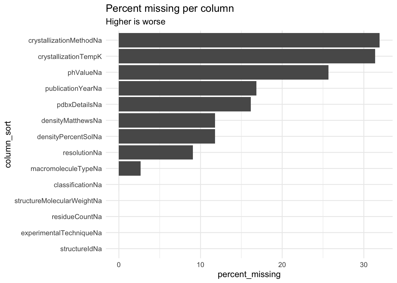
When I looked at the .csv in Excel, I found lots of missing data in the dataset. In this section, I quantify how much missing data there is.
Bar graph of missing value counts
pdb_total_rows = nrow(pdb)

pdb_missing <- pdb %>%
  summarize(
    structureIdNa = sum(is.na(structureId)) / pdb_total_rows * 100,
    classificationNa = sum(is.na(classification)) / pdb_total_rows * 100,
    experimentalTechniqueNa = sum(is.na(experimentalTechnique)) / pdb_total_rows * 100,
    macromoleculeTypeNa = sum(is.na(macromoleculeType)) / pdb_total_rows * 100,
    residueCountNa = sum(is.na(residueCount)) / pdb_total_rows * 100,
    resolutionNa = sum(is.na(resolution)) / pdb_total_rows * 100,
    structureMolecularWeightNa = sum(is.na(structureMolecularWeight)) / pdb_total_rows * 100,
    crystallizationMethodNa = sum(is.na(crystallizationMethod)) / pdb_total_rows * 100,
    crystallizationTempK = sum(is.na(crystallizationTempK)) / pdb_total_rows * 100,
    densityMatthewsNa = sum(is.na(densityMatthews)) / pdb_total_rows * 100,
    densityPercentSolNa = sum(is.na(densityPercentSol)) / pdb_total_rows * 100,
    pdbxDetailsNa = sum(is.na(pdbxDetails)) / pdb_total_rows * 100,
    phValueNa = sum(is.na(phValue)) / pdb_total_rows * 100,
    publicationYearNa = sum(is.na(publicationYear)) / pdb_total_rows * 100
  ) %>%
  pivot_longer(everything(), names_to = "column", values_to = "percent_missing") %>%
  arrange(percent_missing)

pdb_missing %>%
  mutate(
    column_sort = factor(
      column,
      levels = pdb_missing$column
    )
  ) %>%
  ggplot(aes(x = column_sort, y = percent_missing)) +
    geom_col() +
    coord_flip() +
    labs(
      title = "Percent missing per column",
      subtitle = "Higher is worse"
    )
What if I dropped all NA?
Percentage observations remaining if all rows that have NA were dropped:
pdb_no_na_count <- pdb %>%
  drop_na() %>%
  nrow()

pdb_no_na_count / pdb_total_rows * 100
## [1] 46.60575Number of observations remaining if all the NAs were dropped.
pdb_total_rows - pdb_no_na_count## [1] 75500Plan of action: drop rows with NA and filter year range
For this exploration, I will simply drop all rows that have any NA variables. I will also restrict the year range to 2000 to 2018.
pdb_clean <- pdb %>%
  drop_na() %>%
  filter(publicationYear >= 2000, publicationYear < 2018)
Exploratory Visualization and Analysis
Publications per macromolecule type, total up to 2018
Only drop the rows that have no macromolecule or publicationYear type.
Overall, it looks like proteins are by far the most dominant molecules being analyzed.
pdb_publication_count_all_time <- pdb_clean %>%
  group_by(macromoleculeType) %>%
  summarize(publicationCount = n()) %>%
  arrange(desc(publicationCount))

knitr::kable(pdb_publication_count_all_time)| macromoleculeType | publicationCount |
|---|---|
| Protein | 60011 |
| Protein#DNA | 2478 |
| Protein#RNA | 1041 |
| RNA | 518 |
| DNA | 430 |
| Protein#DNA#RNA | 137 |
| Protein#DNA#DNA/RNA Hybrid | 31 |
| DNA/RNA Hybrid | 23 |
| RNA#DNA/RNA Hybrid | 17 |
| DNA#RNA | 12 |
| Protein#DNA/RNA Hybrid | 9 |
| Protein#RNA#DNA/RNA Hybrid | 4 |
ggplot(pdb_publication_count_all_time, aes(x = 1, y = publicationCount, fill = macromoleculeType)) +
  geom_col(position = "stack") +
  scale_fill_viridis_d() +
  labs(title = "Number of publications by macromolecule type") +
  ylab("publication count")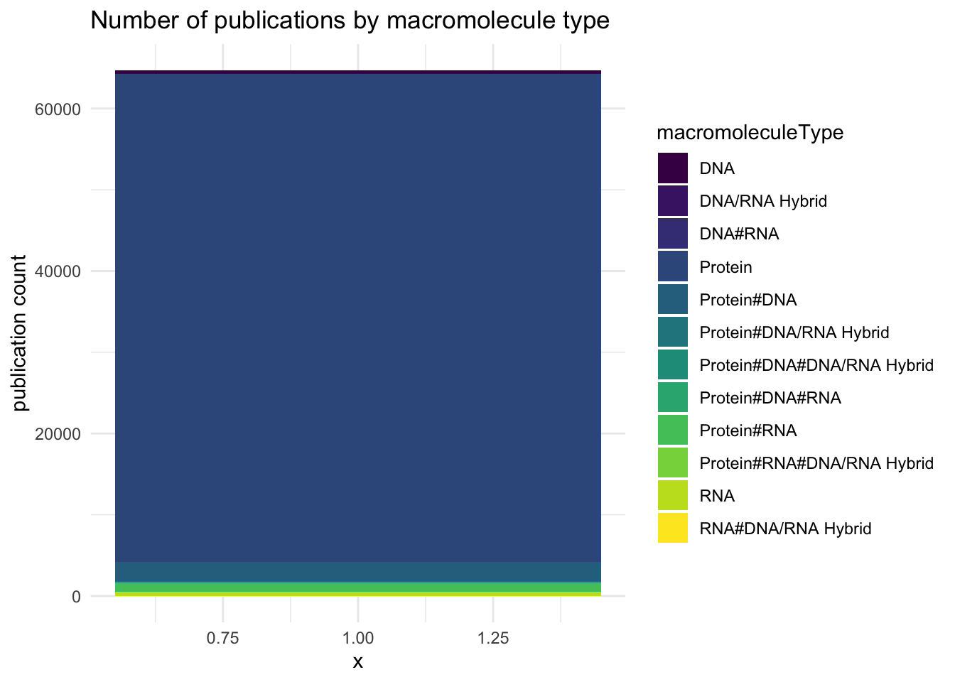
Publications per year, 2000 to 2017
pdb_clean %>%
  group_by(publicationYear) %>%
  summarize(publicationCount = n()) %>%
  ggplot(aes(x = publicationYear, y = publicationCount)) +
    geom_line() +
    labs(title = "Publications per year") +
    ylab("publication count")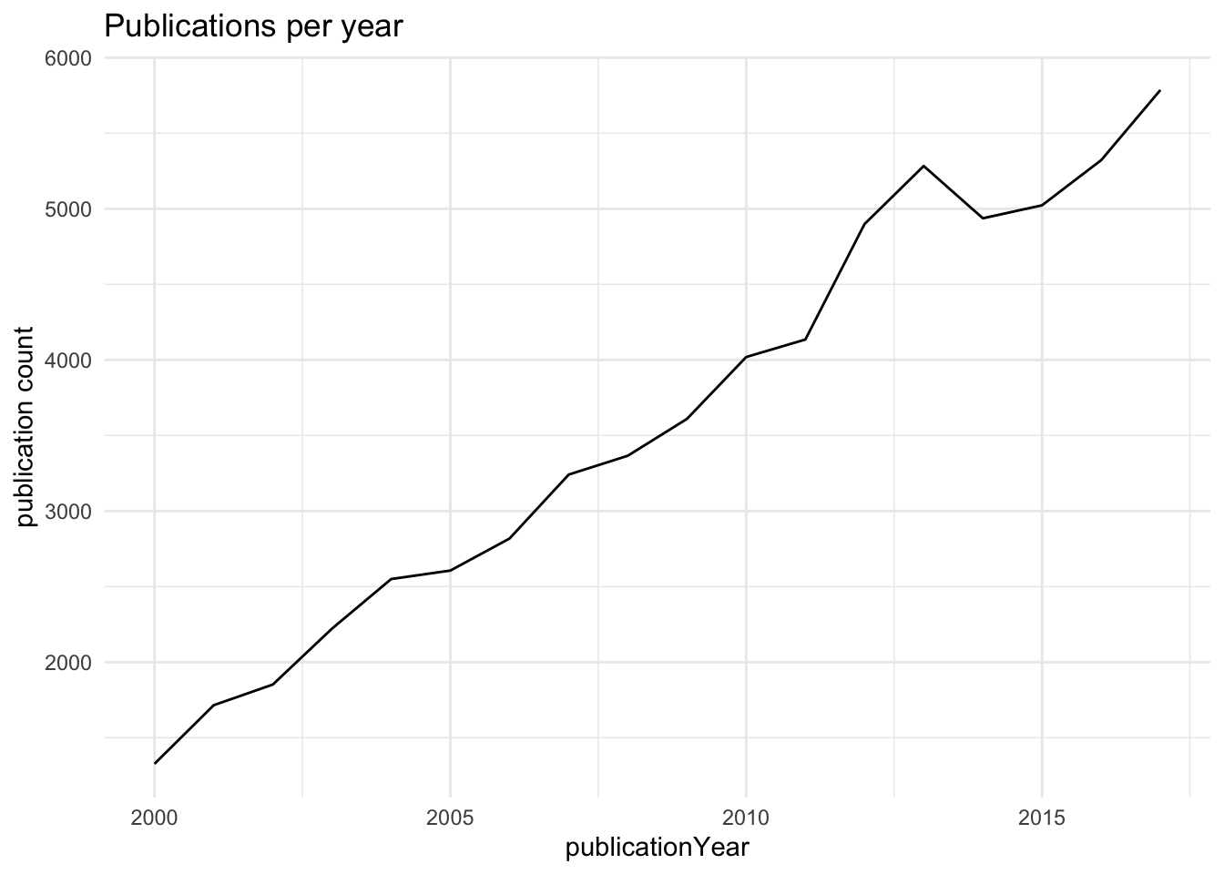
Experimental techniques
Distribution of experimental techniques
Virtually all the publications in the cleaned dataset were from x-ray diffraction.
pdb_techique_counts <- pdb_clean %>%
  group_by(experimentalTechnique) %>%
  summarize(publicationCount = n()) %>%
  arrange(desc(publicationCount))

knitr::kable(pdb_techique_counts)| experimentalTechnique | publicationCount |
|---|---|
| X-RAY DIFFRACTION | 64678 |
| NEUTRON DIFFRACTION | 11 |
| ELECTRON CRYSTALLOGRAPHY | 5 |
| NEUTRON DIFFRACTION, X-RAY DIFFRACTION | 5 |
| POWDER DIFFRACTION | 5 |
| X-RAY DIFFRACTION, EPR | 5 |
| EPR, X-RAY DIFFRACTION | 1 |
| X-RAY DIFFRACTION, NEUTRON DIFFRACTION | 1 |
Molecular weight by experimental technique
It looks like x-ray diffraction has the widest range of molecular weights…but there are far more x-ray diffraction observations in the cleaned dataset.
ggplot(pdb_clean, aes(x = experimentalTechnique, y = structureMolecularWeight)) +
  geom_boxplot() +
  scale_y_log10() +
  coord_flip() +
  labs(
    title = "Molecular weight by experimental technique"
  ) +
  ylab("log(molecular weight)") +
  xlab("experimental technique")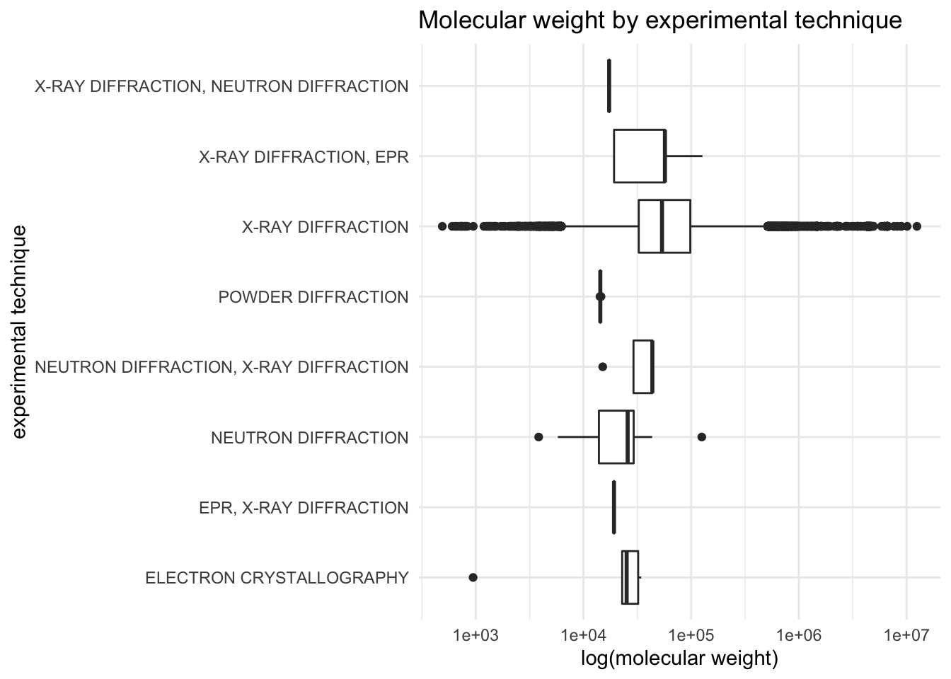
Other variables
Resolution by experimental technique
ggplot(pdb_clean, aes(x = experimentalTechnique, y = resolution)) +
  geom_boxplot() +
  coord_flip() +
  labs(
    title = "Resolution by experimental technique"
  ) +
  ylab("resolution (angstroms)") +
  xlab("experimental technique")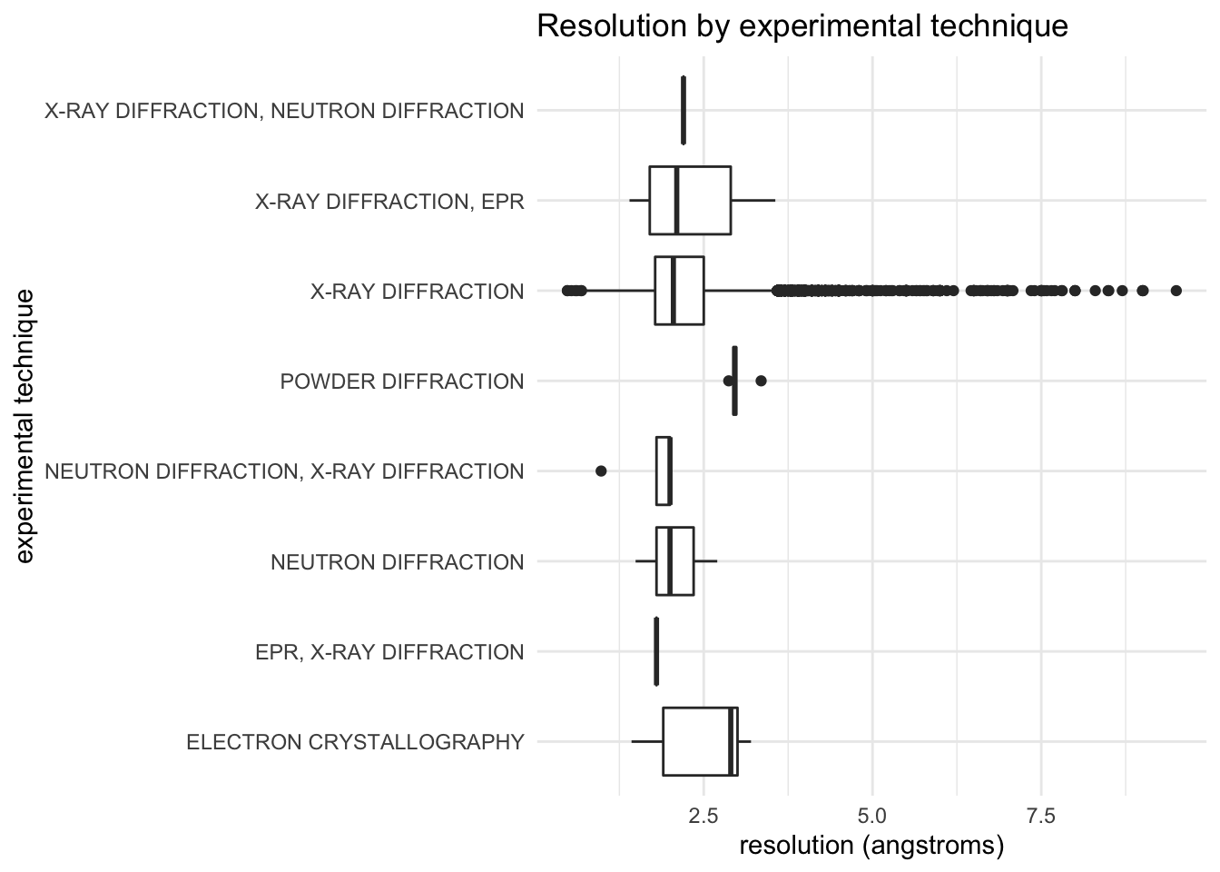
densityMatthews
Mathews density as described in Matthews coefficient probabilities: Improved estimates for unit cell contents of proteins, DNA, and protein–nucleic acid complex crystals.
ggplot(pdb_clean, aes(x = densityMatthews)) +
  geom_histogram(bins = 100)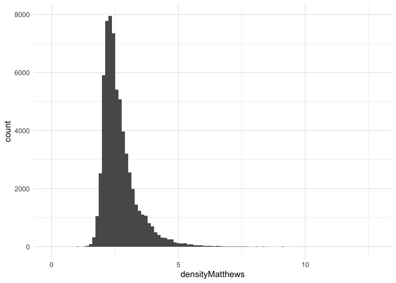
densityPercentSol
I wonder if these could be tied back to crystallization methods or crystallization temperature.
ggplot(pdb_clean, aes(x = densityPercentSol)) +
  geom_histogram(bins = 100)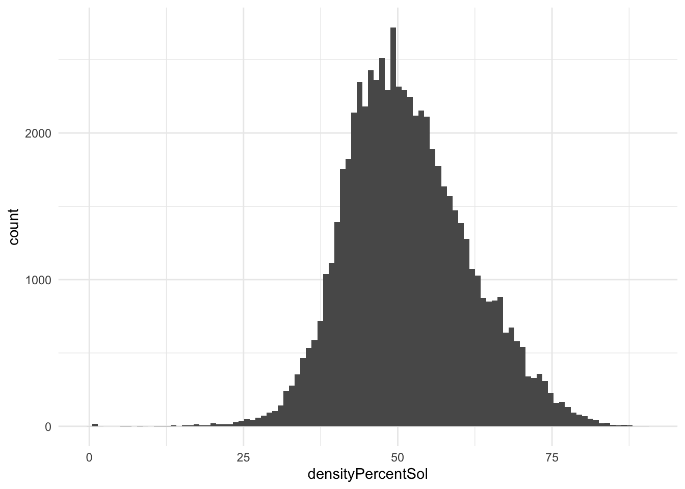
Classification column
For this section, only apply cleaning to the classification column.
Top classifications
What are the top 10 classifications?
top_classifications <- pdb_clean %>%
  group_by(classification) %>%
  summarize(classification_count = n()) %>%
  arrange(desc(classification_count))

knitr::kable(head(top_classifications, 5))| classification | classification_count |
|---|---|
| HYDROLASE | 10090 |
| TRANSFERASE | 7583 |
| OXIDOREDUCTASE | 6109 |
| IMMUNE SYSTEM | 2397 |
| LYASE | 2290 |
Conclusion
In the future, it would be interesting to:
Train a model on the sequence data that accompanies this dataset, to see if I could fill in missing values based on sequence data.
Find if there were any systematic features missing for each
macromoleculeType. Maybe each macro molecule should get its own schema of attributes that are likely to be filled in.Mine the text of
pdbxDetails. Perhaps these could correlated with things like ph, resolution, experimental method, etc.Mine the text of
crystallizationMethod. Perhaps these could correlated with things like ph, resolution, experimental method, etc.Mine the text of
classificationsince there are so many unique values in that column.